1. INTRODUCTION

With the advent of the New Space era, the number of artificial space objects orbiting Earth has been increasing exponentially [1]. In particular, Low Earth Orbit (LEO) has become highly congested due to the concentration of satellites for various purposes such as communication, Earth observation, and environmental monitoring. Consequently, the risk of satellite collisions and atmospheric reentry is escalating [2]. Furthermore, the expansion of military satellite operations demands national capabilities to counter space threats from intentional maneuvers and malicious approaches [3]. We are now facing technological challenges for national security, space traffic management and the long-term sustainability of space activities.

Space surveillance encompasses the detection, tracking, identification, and cataloging of space objects and is broadly classified into Space Situational Awareness (SSA), which focuses on ensuring space safety through positional predictions, and Space Domain Awareness (SDA), which aims to characterize intentions and respond to military threats [4].

Various sensor systems are utilized to establish surveillance networks: radar, optical, radio frequency and laser-based technologies. Depending on the characteristics of each sensor, some systems are effective for uncued surveillance, while others require prior target information.

In South Korea, the Korea Astronomy and Space Science Institute (KASI) has been operating the Optical Wide-field Patrol Network (OWL-Net) [5]. OWL-Net consists of 0.5m optical telescopes deployed across five countries, monitoring national space assets in both LEO and GEO, and is capable of making orbit determinations. However, due to its limited field of view (approximately 1.1° × 1.1°), OWL-Net is primarily suited for tracking satellites with known orbits. This limitation makes it nearly impossible to characterize uncatalogued space objects or satellites that may pose threats to national assets. Optical systems are also highly susceptible to weather and sunlight conditions. For these reasons, there has been significant interest in the development and deployment of a radar surveillance system in South Korea [6]. The Republic of Korea Air Force (ROKAF) is also pursuing a radar surveillance system as an important part of its future SDA framework. Weather-independent, real-time detection of both known and unknown LEO space objects passing over South Korea will make it possible to produce and maintain our own space object catalogs [7].

However, space surveillance based solely on a single radar station has inherent limitations in coverage and continuous monitoring. This is because only a small part of the LEO volume can be observed at any given time. For this reason, it is always beneficial to place SSA sensors globally to increase observation frequency and coverage. The most well-known space surveillance system, the United States Space Surveillance Network (SSN), is one such example. Originally developed for ballistic missile tracking, SSN’s radar systems around the world have since been adapted for LEO space object surveillance [8]. Recently, two new Space Fence radars have been added to the SSN, significantly enhancing its ability to track smaller space objects in LEO [9]. Radar systems currently cannot perform effectively beyond the LEO volume; therefore, SSN’s optical telescope network has been responsible for space objects at higher altitudes including GEO satellites.

This study aims to understand the capability and limitations of a single Space Fence type two-dimensional phase array radar system (2D radar hereafter) to be built in South Korea. We then explore how to improve its SSA capability through an additional complementary network of global sensors. Two possibilities are considered. The first option is a network of affordable radar systems similar to LeoLabs 1-dimensional space radars (1D radar hereafter). These 1D radars do not track but still produce useful detection data to improve orbit information [10]. We assume a situation where we build our own network or purchase observation-level data from existing systems. The second option is a network of wide-field optical sensors for uncued large area surveillance. Optical telescopes for LEO are often used to track known objects due to their very limited field of view (FOV), and are therefore not very effective for general surveillance. However, the high sensitivity of recently developed CMOS sensors combined with large FOV optics makes it possible to cover a large portion of the sky with both detection and tracking capabilities. Optical SSA based on the so-called Ultra Wide Field-of-View (UWFoV) system has been shown to be very effective for general surveys [11]. Due to its low cost and ease of installation, it is also quite feasible to build a relatively large global network.

The remainder of this paper is organized as follows. Section 2 describes our numerical simulation methods, the virtual satellites used in the experiments and the simulation environment. Section 3 evaluates the efficiency and limitations of a single 2D radar station to be deployed in South Korea. Section 4 addresses cases of a complementary network, where multiple 1D radars or UWFoV optical surveillance systems are deployed at various international sites. Section 5 examines the impact of weather conditions on optical surveillance and Section 6 presents our conclusions.

2. NUMERICAL APPROACH FOR SATELLITE OBSERVATION FREQUENCY

2.1. Simulation Strategy

We employ numerical simulation techniques to analyze the performance of the surveillance system and to compare cases of a single system with complementary global networks. The primary metrics of survey performance are revisit time and daily detection frequency. Revisit time refers to the time interval between successive detections of a given space object and, in our case, is calculated based on the satellite’s culmination over each sensor’s visibility window.

The simulation is performed for a seven-day period with a large set of virtual space objects, whose orbits are propagated using NASA’s SGP4 propagator within the Skyfield library [12]. Three different altitude groups of virtual samples are considered: 250 km, 550 km and 1200 km, so that we can study the survey efficiency dependence on target altitudes. Skyfield provides the time and location of rising, culmination, and setting of each space object over a given elevation for each assumed sensor site.

It should be noted that we do not consider radar power, optical sensitivity, satellite size or radar cross-section (RCS). The detectability of satellites is determined solely based on whether they pass through the sensor’s field of view. For optical systems, we consider additional factors such as the distinction between day and night as well as the effect of sunlight reflection. Specifically, we define the nighttime observation window based on civil twilight, where the Sun is below -6° in elevation, and use Skyfield’s sunlit function to determine sunlight reflection conditions.

2.2. Virtual Satellites for Simulation

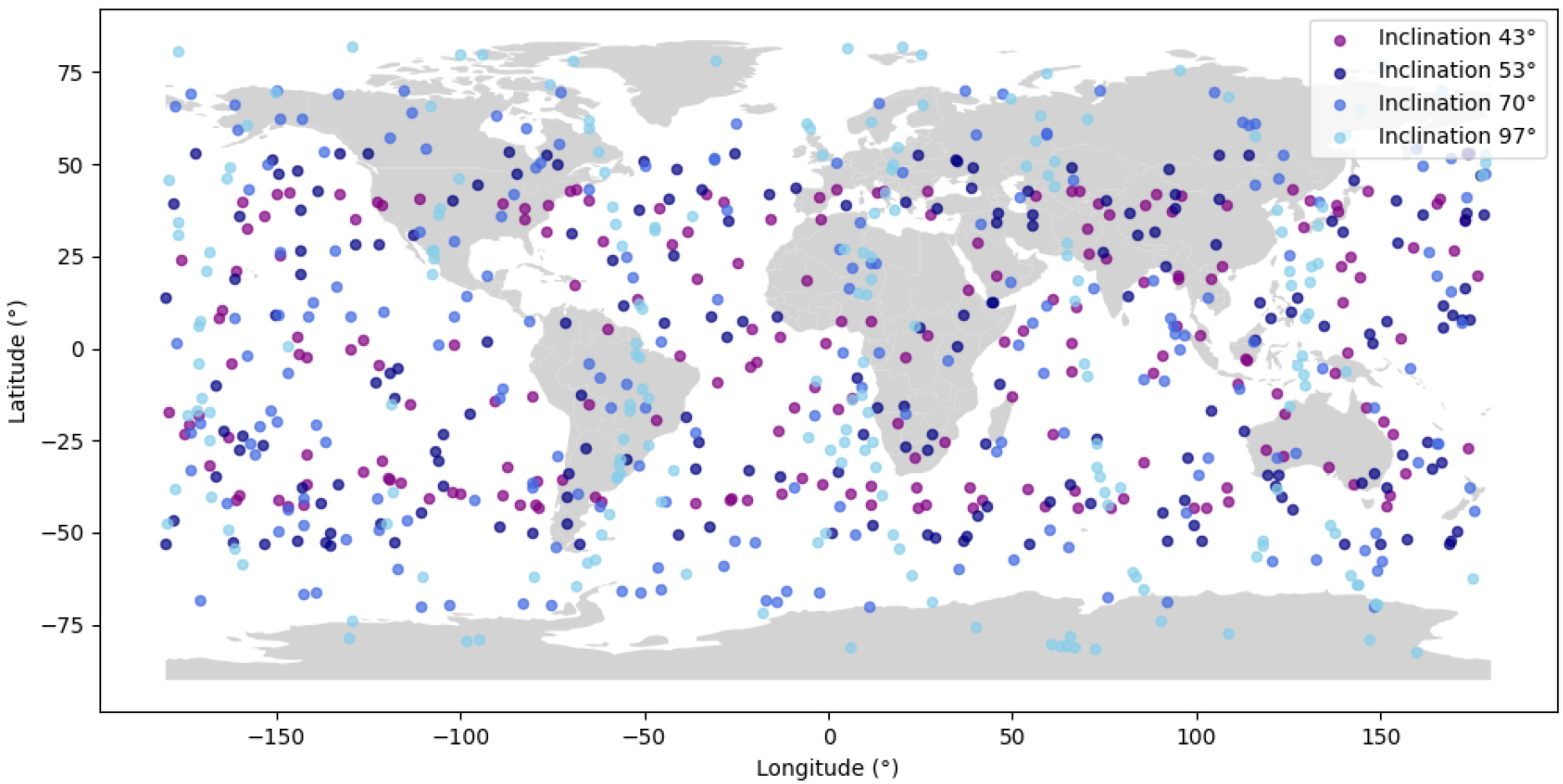
We select our initial samples from the Starlink constellation, which consists of a large number of satellites with rather uniform distribution. The average altitude of Starlink satellites is approximately 500 km, making it the most congested volume. It is therefore natural to select our 550km population from the existing Starlink satellite database of TLE data provided by Space-Track [13]. The 800 selected satellites are shown in Fig. 1. They have altitude ranges of 530-550 km with four groups of orbital inclination: 43°, 52°, 70° and 97°. For each orbital plane, 200 randomly selected satellites are assigned to different Right Ascension of the Ascending Node (RAAN)values.

FIG. 1.

800 Starlink satellites of our 550km population are shown. We consider four inclination groups, each consisting of 200 randomly selected from Starlink satellite TLE entries of Space-Track.

Very Low Earth Orbit (VLEO) generally refers to orbits below 400 km altitude. There are only a few satellites operating in VLEO at present due to extremely large atmospheric drag. However, VLEO is likely to become a very busy volume of space in the near future for next generation satellite communication, high-resolution Earth observation, as well as military reconnaissance purposes. Given its increasing potential for widespread utilization, we believe it is important to estimate the VLEO survey efficiency and therefore have prepared the 250 km population.

This 250 km population can also serve as a measure of re-entry monitoring capability. Without active propulsion, space objects in LEO will eventually re-enter the atmosphere. Once satellites or rocket bodies begin their re-entry, they become objects of concern because of the potential damage they could cause in commercial air space and on the ground. It is very difficult to predict locations of re-entry and ground impact. Frequent observations in the VLEO region until they reach the upper atmosphere are necessary to improve predictions, and the survey efficiency of this 250km population can be a useful measure of this type of surveillance.

We derive our 250 km sample from the 550 km sample of Starlink satellites, by adjusting the mean motion so that the orbital altitude becomes 250 km. For each satellite, we apply the following Eq. (1)[14]:

where G represents the gravitational constant, M is the mass of Earth, R is the Earth’s radius, and h is the desired altitude in kilometers. We set external perturbations to zero to simplify the calculations. This is achieved by setting the eccentricity, 1st derivative, 2nd derivative, and B*drag terms in the TLE to zero, making them pure circular orbits. Note that our simulation does not intend to follow atmospheric drag in detail, but to estimate the detection frequency over a seven-day period. In order to examine surveillance efficiency for higher LEO altitudes, we also apply the same procedure to generate a synthetic satellite population at 1,200 km. This allows us to conduct quantitative assessments of surveillance performance across different orbital altitudes of 250, 550 and 1200 km.

3. CASE OF SINGLE 2D RADAR AND ELEVATION

3.1. Spatial Coverage and Elevation

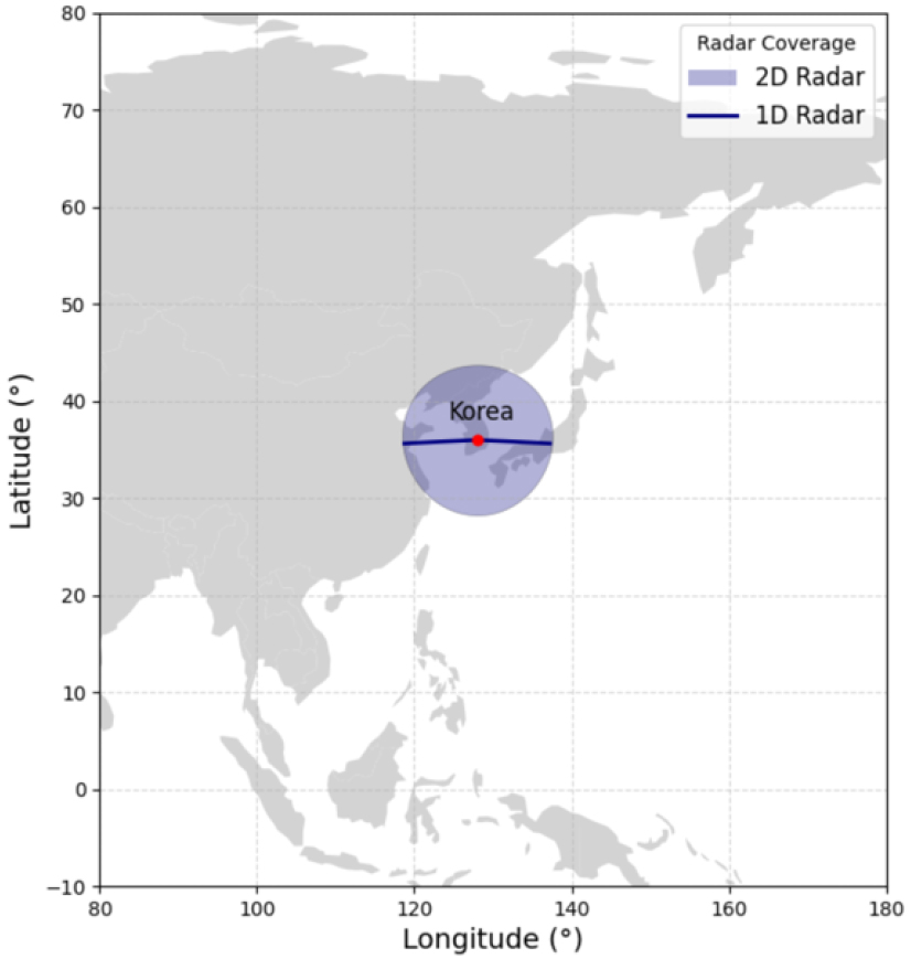
The specification of the South Korean space surveillance radar system is not determined yet. We therefore assume that it is capable of 2D detection and tracking in all directions above an elevation angle of 30°. This reflects the fact that most phase-array radar has a field of regard of 120°. In Fig. 2, we show the coverage area of this 2D radar system for 550 km altitude. For comparison, we also mark the coverage of a LeoLabs type 1D linear array radar whose structure is aligned in the East-West direction. With the elevation limit of 30°, the coverage naturally becomes larger for higher altitudes and smaller for lower altitudes.

FIG. 2.

Surveillance coverage virtual 2D and 1D radars located in South Korea, for space objects of 550km altitudes and an elevation limit of 30°.

The sensor’s elevation limit affects detection frequency greatly. We can visualize this by showing the distribution of all culmination events in the space of azimuth and elevation. Fig. 3 presents this culmination statistics for the 550 km sample passing over South Korea during a seven-day period. Higher culmination frequencies are represented by brighter colors, and it is shown that the number of culmination events is significantly higher at lower elevation angles. For instance, among all satellites with inclinations of 53°, 70°, and 97° passing above 10° elevation, less than half reach culmination at an elevation angle above 30°, and only about a quarter exceed 50°.

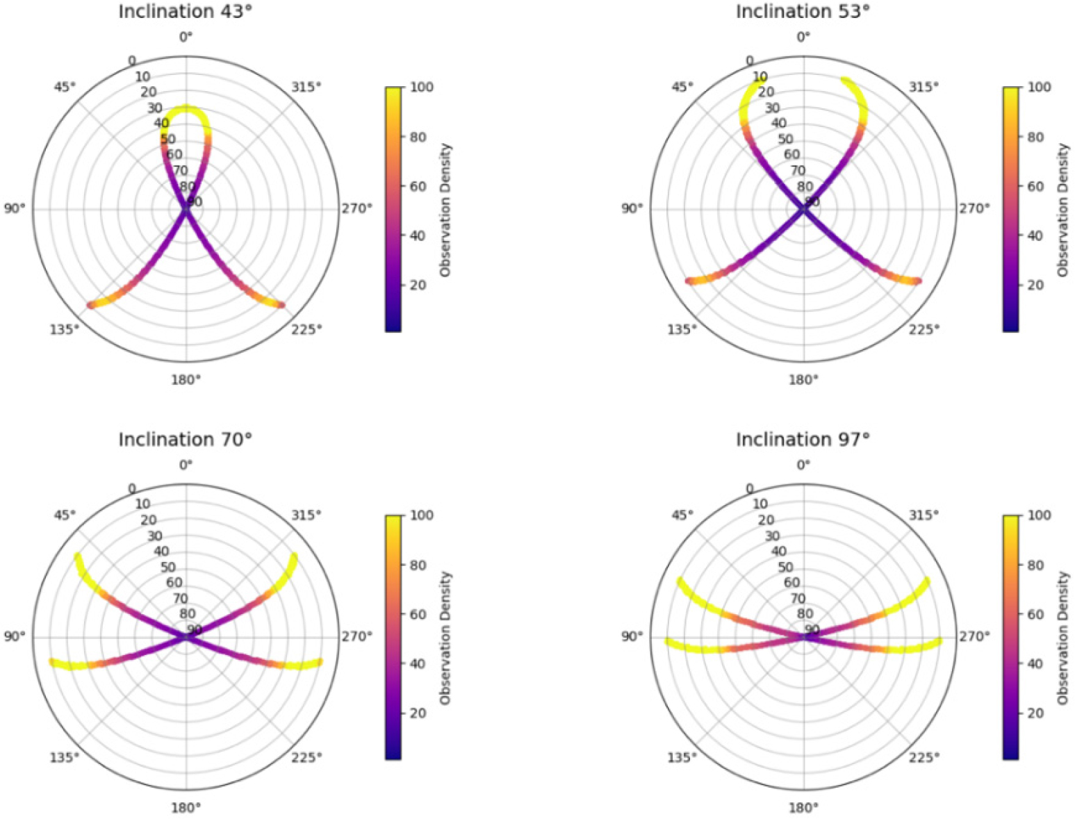
FIG. 3.

Culmination locations of 550 km satellite population observed from Korea, categorized by orbital inclination. Azimuth and elevation angles are marked. Kernel Density Estimation (KDE) are used to show observation density of satellites. More satellite passes happen at lower elevations and low inclination satellites (especially 43° group) show orbital caustic effect in northern skies.

The situation is somewhat different for satellites with an orbital inclination of 43°. Culmination passes are densely concentrated in the northern sky at elevation angles between 30° and 45°. Among the satellites that pass above 10° elevation, three quarters of culminations occur at elevations above 30°. This is due to the orbital caustic effect, occurring when satellites traveling along an inclined orbit pass through a latitude turning point. This leads to increased orbital overlap in our northern sky, which can be detected by the 2D radar system considered here.

3.2. Observation Frequency and Revisit Time

LEO satellites orbit the Earth 15 or 16 times per day. However, the chance of observing a satellite from a given site depends on the surveillance sensor’s field of view, the satellite’s altitude and orbital inclination. Fig. 4 illustrates how the average daily surveillance frequency varies under these conditions. The results indicate that as the satellite altitude increases, the number of observations also increases, reflecting the fact that the survey volume becomes larger for higher altitudes. Additionally, satellites with lower orbital inclinations are observed more frequently due to their denser ground tracks, as they pass over a relatively smaller portion of the Earth’s surface. Fig. 4 also shows that at an altitude of 550 km, satellites with an inclination of 43° are observed more frequently by the 2D radar system compared to the 1D system. A similar trend is observed for the 1,200 km group, where differences in observation frequency persist for 43° and 53° inclination satellites. This phenomenon is attributed to the orbital caustic effect, as previously discussed. The 1D radar with East-West configuration detects only those satellites that cross the East-West line and therefore cannot observe the caustic effect.

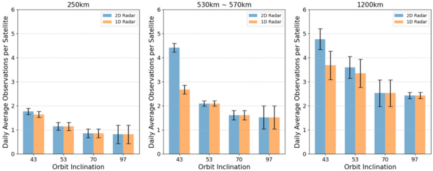
FIG. 4.

Average number of observations per satellite per day at a Korean site, for three altitude populations and different inclination groups. Lower altitudes are more difficult due to smaller survey volume regardless of sensor types.1D radar configured for East-West direction does not benefit from the orbital caustic effect for 43° inclination group.

In most cases, satellites are observed once or twice per day. At lower altitudes, however, some satellites are observed much less. Approximately 8% of satellites are observed fewer than three times during the seven-day period. Each detection, especially with the tracking-capable 2D system, will help improve orbital information of previously known objects. However, the observed track of an LEO object corresponds to a small portion of an orbit and therefore its usefulness for initial orbit determination is limited. Re-observation and association are necessary to derive reliable orbit information and maintain orbit catalogs of higher accuracy. If the re-observation happens many orbits later, then it becomes difficult to associate and derive good orbits. The same is also true for maneuver detections.

For this reason, a good surveillance system aims to have smaller revisit time statistics. We calculate the revisit time for every sample satellite during the seven-day period and visualize it in Fig. 5. It can be seen that for the 250 km group, the time between consecutive observations varies widely, ranging from approximately 4 hours to more than 24 hours. This suggests that, even when a satellite is observed twice a day, some are revisited within a few hours while the majority require many orbits before being observed again. At 550 km, the frequency of short revisit times increases. Some satellites are observed immediately after completing one full orbit, representing an ideal case for establishing good orbit estimates. However, most satellites require several hours and in some cases are not detected again within 24 hours. The 1,200 km sample shows improved revisit time statistics. The average revisit times, with very large dispersions, are 18, 9.4, and 7 hours for 250, 550, and 1200 km samples, respectively.

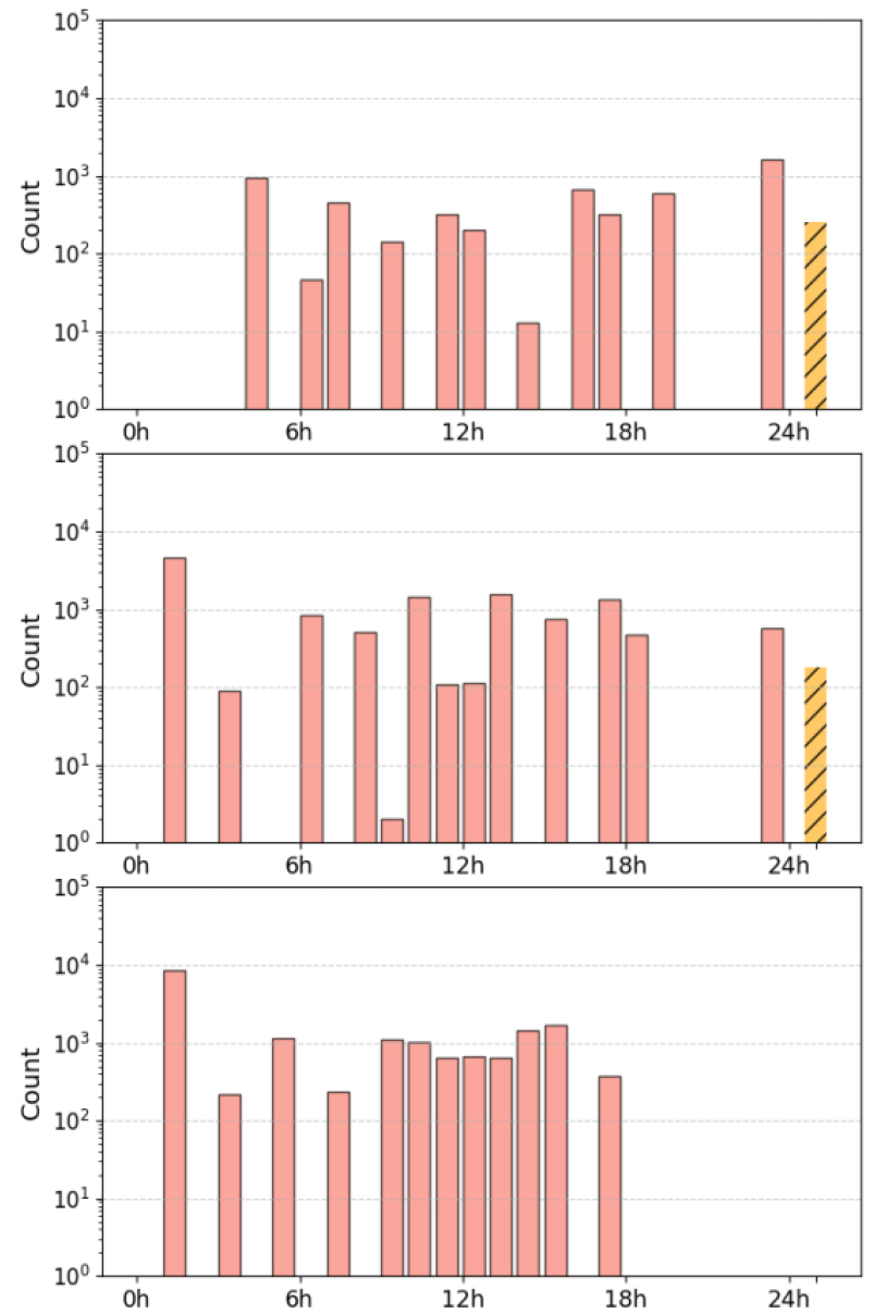
FIG. 5.

Revisit time of a single 2D radar site. Each panel shows samples of 250, 550 and 1,200 km altitudes from top to bottom. The x-axis represents the revisit time, while the y-axis shows the number of observations for a seven day period. The yellow bars indicate the number of satellites that are observed once and then re-detected after 24 hours.

Long revisit times indicate rather limited response capability for satellite maneuvers and also for re-entry objects with continuously decaying orbits. VLEO satellites are likely to use propulsion systems frequently, and frequent observations will facilitate association and orbit updates. The situation would certainly improve if we were to develop and operate multiple 2D radar systems in global locations. This is unlikely to happen, however, due to the high cost of installation as well as geopolitical difficulties concerning military applications of space surveillance.

4. COMPLEMENTARY GLOBAL SENSOR NETWORK

The improvement of the 2D radar’s surveillance efficiency is possible through two approaches. One approach is to lower the elevation angle limit below 10° by employing more than one phased array radar or by configuring the array to have a curved surface. As discussed in the previous section, this alone could nearly double the number of satellites detected by the system through a much larger surveillance volume. However, the ultimate enhancement is possible by combining data from a global network of sensors. One potential solution is to acquire SSA data from either allied nations or international commercial entities. Data sharing is already active for many unclassified space objects through Space-Track, but is unfortunately limited to TLE information. There have been discussions on how to improve international cooperation on space traffic management by exchanging observation-level SSA data and common analysis tools, but it is considered challenging as a state’s SSA infrastructure has both civilian and military components. The latter often concerns national security [15]. While the most useful method of data integration is to combine raw observation data, it is unlikely to happen as such a level of data exchange would expose the full capability of surveillance systems.

We therefore consider two other possibilities. One is to purchase observation data from a commercial company that operates a network of cost-effective 1D radars. Another is to build our own network of UWFoV optical sensors. This optical system can be built and operated without significant investment and its small footprint allows relatively easy installation. As claimed by a recent commercial operational example, UWFoV optical systems can produce millions of uncued detections and trackings every night [16].

Table 1 lists the sites of complementary sensors used in this study. For the 1D radar, we simply use the locations of LeoLabs space radars. For UWFoV optical sensors, we have chosen extra locations where we already have national research facilities with a good possibility of hosting a small composite camera system such as the proposed sensor. The site locations are shown in Fig. 6 with each UWFoV sensor’s surveillance area indicated by a set of shadows. The coverage depends significantly on target altitudes, but the figure already shows the benefit of having a large network across the globe.

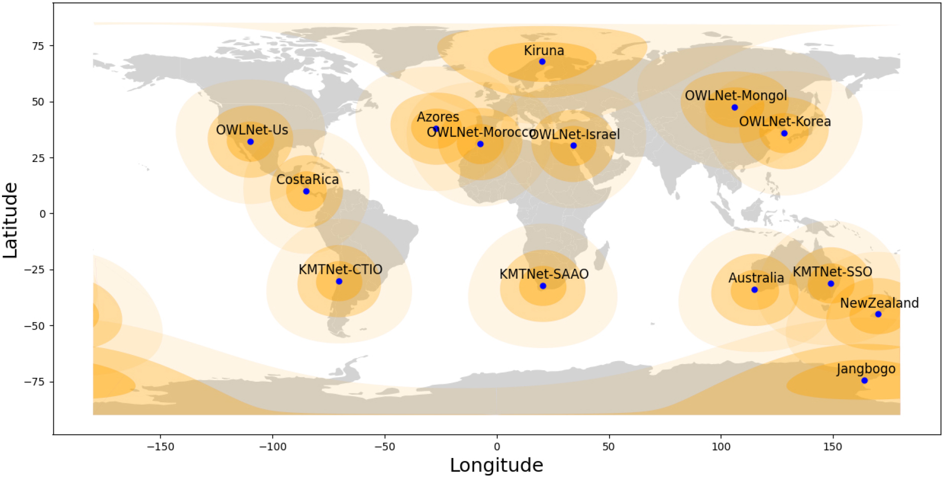
FIG. 6.

Geographical distribution of assumed global sites for 1D radars and optical system, also listed in Table I. Surveillance areas for UWFoV systems (with elevation limit of 10°) are marked by circular shades. From the innermost to the outermost, the regions corresponds to target altitudes of 250, 550, and 1,200 km.

4.1. 1D Radar Network

We consider the case where four 1D radars at international locations supply their SSA data. LeoLabs space radars in Australia, New Zealand, Costa Rica, and Azores are included. Each of these radars has two 1D arrays in parallel or in cross configuration. A detection is confirmed when it happens in both arrays. Our simulation follows this logic as well. More details can be found in the LeoLabs publication [17].

The left panels in Fig. 7 show the average number of daily observations per satellite when our 2D radar is aided by data from these four 1D radars. It can be seen that satellite detection rates do increase, but the improvement depends on the altitude of satellites. The 550 km and 1,200 km samples are observed several times per day, and for low inclination groups over 10 times. The 250 km samples are, however, still observed much less. We note that high inclination groups are consistently less frequently observed for all altitude samples. The left panels of Fig. 8 present the revisit time distribution. The average revisit time for satellites at 550 km decreases to 2.7 ± 2.5 hours. At 1,200 km, the revisit time is reduced to 1.8 ± 1.8 hours, while at 250 km, it decreases to 5.0 ± 3.9 hours (see Table 2). Compared to the 2D radar system alone (Fig. 5), the revisit time distribution shifts significantly toward shorter intervals.

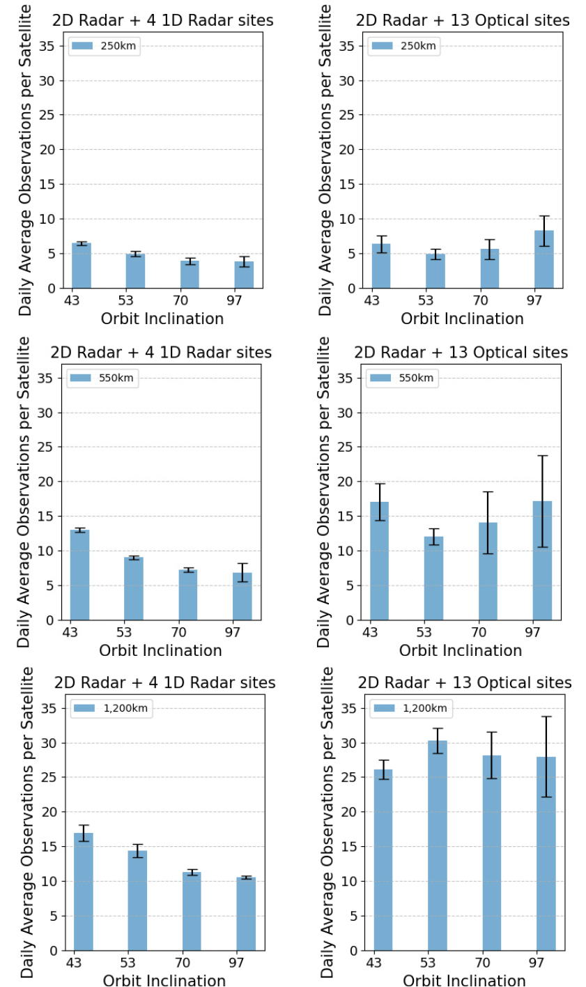
FIG. 7.

Comparison of the average daily number of observations per satellite when four additional radar sites and thirteen optical sites are added to a single 2D radar site. From top to bottom, the assumed altitudes are 250 km, 500 km, and 1,200 km. Adding thirteen wide-field optical systems with an elevation angle of 10° or higher allows for the observation of more satellites compared to adding four 1D radar sites.

We assume here that every detection the 1D radar makes is useful in identifying and updating the satellite’s orbit. The lack of tracking information, however, is likely to present a challenge in association [18].

4.2. UWFoV Optical Sensor Network

Optical surveillance systems operate at night and detect only those satellites passing through the region that can reflect sunlight. Due to these limitations, we consider deploying a larger number of optical sensors, as their operational opportunities are significantly more limited than those of radars. These sensors can be designed for all-sky coverage, but considering the low transparency near the horizon, we set the elevation limit at 10°. The optical system can perform simultaneous detection and tracking of multiple objects without prior orbit information. The same data can also be used to analyze satellite brightness variations and therefore to determine the real-time rotational states of satellites [19].

When integrated with a 2D radar system, the UWFoV optical network significantly enhances the SSA capability. The right panels of Fig. 7 show the cases of thirteen UWFoV optical systems operating together with the 2D radar system. The daily average number of observations per satellite increases by five times or more; the benefit is greater for higher altitude groups. It can be seen that the UWFoV results are always better than the cases of four 1D radars. The improvement is most apparent for polar orbit satellites. This is likely due to the low elevation limit given to the optical sensors as well as the presence of polar sites.

The right panels of Fig. 8 show the distribution of revisit times. Thirteen UWFoV sensors provide much better revisit statistics than a single 2D radar. The improvement is also better than the case of four 1D radars. While optical systems have serious limitations regarding observation windows and sunlit conditions, it appears that the large number of sensor deployments is sufficient to overcome such limitations.

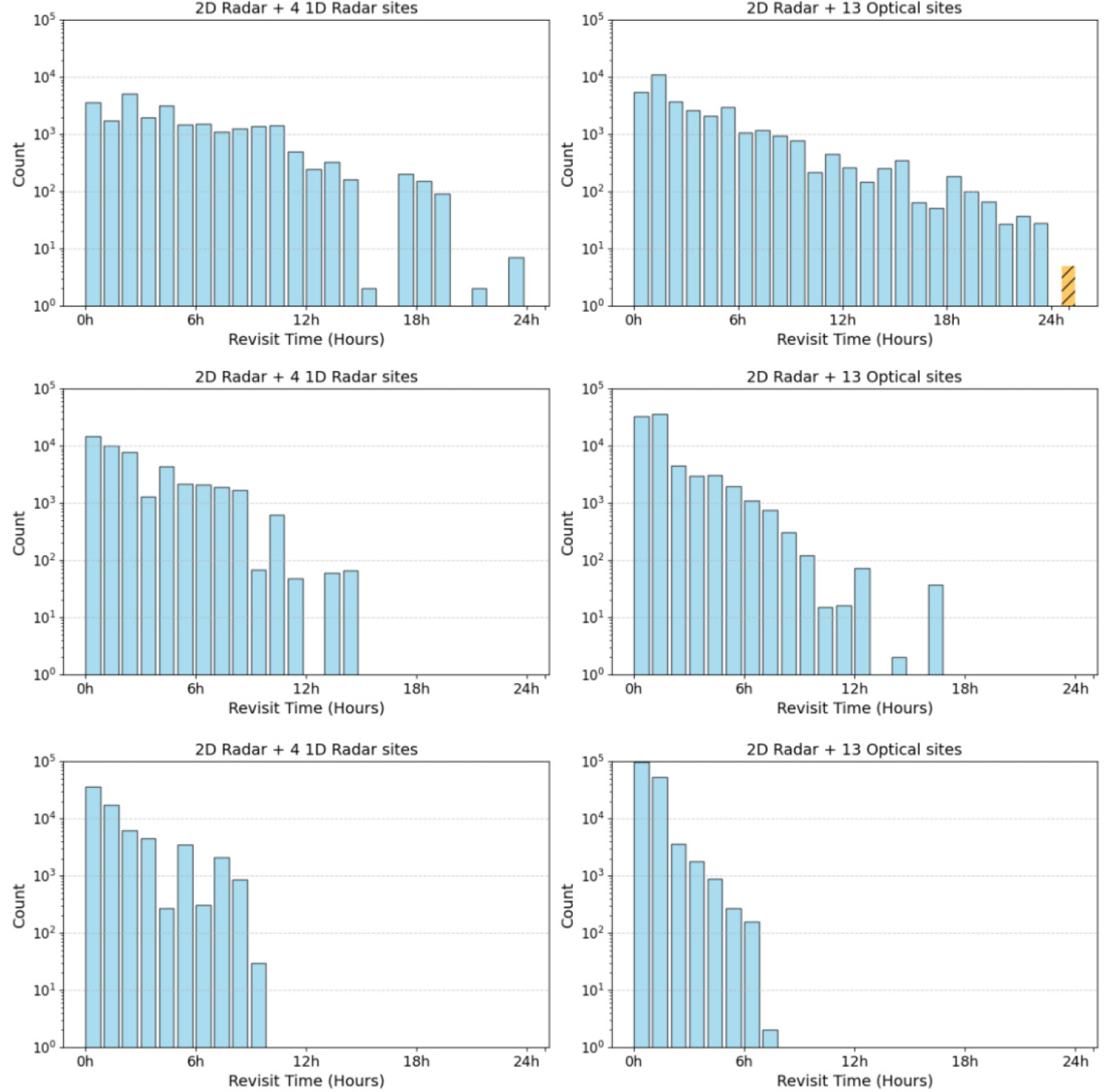
FIG. 8.

Comparison of revisit time when four additional radar sites and thirteen optical sites are added to a single 2D radar site. From top to bottom, the assumed altitudes are 250 km, 550 km, and 1,200 km. At 250 km, even after adding thirteen optical sites, there were cases where some satellites were not observed more than once within 24 hours.

Our results of average revisit time are summarized in Table 2. For the 550 km sample, the revisit time of 9.4 hours for the 2D radar improves to 2.7 and 1.5 hours when either four 1D radars or thirteen optical sensors are added respectively. We note that this means we can update the orbit of these satellites almost every orbit or every other orbit, allowing very early detection of maneuvers and any significant orbit changes. For the 1200 km sample, this number becomes less than an hour. The VLEO 250 km sample remains the most challenging even with the addition of global sensors. While the average revisit time improves from 18 hours to 5 or 3.7 hours, a large fraction of revisits occurs after 12 hours. Table 2 also shows the statistics for polar orbit satellites.

Polar orbits have the advantage of global coverage and are often utilized by Earth observation and information gathering missions. It can be seen that the revisit time of polar orbits is much worse than others when we have only a single 2D radar system; almost 15 hours for the 550 km sample. This improves greatly when we have complementary systems of global deployment; 3.3 and 1.5 hours for the 550 km sample, when aided by the 1D radars and optical networks respectively. The optical network appears to be the most effective in reducing the revisit time for these polar satellites, and as in the case of daily number of observations, we believe this results from the low elevation limit and the presence of polar sites in the assumed optical UWFoV network.

5. WEATHER IMPACT ON OPTICAL NETWORK

5.1. Collection of Weather Statistics

Ground-based optical sensors cannot operate in bad weather when stars and satellites are not visible. Our numerical simulation for optical sensors does not consider this, and therefore we need to estimate the influence of weather.

There are several archival databases for global weather information with many weather parameters, but we have chosen to use the Cloud Cover (CC) parameters. CC represents the percentage of the sky covered by clouds, where 0% indicates clear sky conditions and 100% indicates a fully overcast sky. A recent and comprehensive study on this subject presents monthly average CC values for many astronomical observatory sites around the world using data collected for a period of 20 years from 2000 to 2019 [20]. Some sites in Table 1 (Azores and polar locations) are unfortunately not included in this publication, and we use data from another study [21] where seasonal variation of CC is analyzed for approximately a 30 year period between 1952 and 1981. We have combined the results of these two studies and the variation of monthly CC values for the 14 sites in Table 1 is shown in Fig. 9.

FIG. 9.

Monthly Cloud Cover for our virtual surveillance sites as derived from [20] and [21].

5.2. Influence on Revisit Time Estimates

The numerical calculation in this study is conducted for a seven-day period in March 2025, and therefore we have used the March CC information to correct the detection records of optical sensors for each site. This corresponds to nearly 50% of data cancellation overall.

The estimated revisit times naturally increase compared to the values given in Table 2. For the 550 km sample, the revised average revisit time is 2.8 ± 2.9 hours, about twice longer than the original. The revised times for 250 and 1200 km samples are also doubled to 7.1 ± 6.9 and 1.5 ± 1.4 hours, respectively. This is a natural consequence of removing half of the observation data from the optical network.

We note that the optical revisit time statistics are still comparable to those of the 1D radar case even considering the CC influence. Therefore, while weather does significantly impact the survey efficiency of optical sensors, we conclude that a global network of UWFoV sensors offers an important opportunity to improve the SSA capability of a single 2D radar system.

The CC distribution in Fig. 9 also demonstrates that there are substantial differences among the sites. It is clearly very important to find optical sites with superior CC conditions. We also need to consider adding extra sites to maximize overall operation rates throughout the year as pronounced seasonal CC changes are apparent at several sites. It would be possible to run a year-long SSA simulation focusing on the CC-considered performance of many more potential sites worldwide, but this is beyond the scope of the present study.

6. CONCLUSION

Our study evaluates the surveillance efficiency of SSA for LEO objects. For three altitude groups of virtual satellites at 250, 550 and 1200 km, we calculate the daily number of observations and revisit time statistics for different sets of sensor configurations. Three cases are considered: a single 2D radar located in South Korea, and when this facility is aided by additional data from a global network of four 1D radars or by a larger global network of thirteen UWFoV optical sensors.

Our findings demonstrate that the presence of global sensors greatly improves the number of observations. Even with limited operation windows and dependence on sunlit conditions, we find that the optical sensor network represents a highly attractive solution to minimize the revisit time most effectively. For space objects at 550 and 1200 km altitudes, this means that their orbits can be examined for unexpected maneuvers and other orbit changes almost every orbit. Effective SSA remains challenging for the VLEO 250 km sample due to the smaller surveillance volume at low altitudes, but both observation frequency and revisit time improve with the aid of complementary networks.

Optical SSA from the ground cannot operate through clouds and we have found that the impact can easily remove half of the observational data when average CC effects are applied to each of the optical sites. Nevertheless, the weather-affected optical data exhibits better or similar performance when compared to the global network of 1D radars.

Our conclusions are as follows. A new Space Fence-like 2D radar will be an important step forward for Korean space security and for global space sustainability. However, the operation of a single 2D radar is limited by its small surveillance volume, which results in sparse observations and long revisit times. The system will have limited capability to detect orbit changes and will suffer from association difficulties for new objects. The optimal solution to these problems is to obtain observational-level data from global locations. This study demonstrates precisely how much improvement can be expected from different configurations of complementary global systems. Several 1D radars at international locations provide meaningful enhancement, while the deployment of many more UWFoV optical sensors proves to be even more effective.

It may be possible to access shared data from allied facilities or to purchase it from commercial entities, but such data will most likely be provided in the form of processed data rather than observational data due to security considerations. Therefore, it is probably the most prudent approach to establish our own global network of small sensors, which will eventually operate in conjunction with the Korean space radar. We note that the data processing and object association technologies developed in the process will also become important assets for space-based SSA to be realized in the near future.